Before we start, I have to clarify, this is not a way of “hacking” TLS to decrypt any encrypted traffic! This is (probably) not possible. What we will do in this tutorial is to temporarily extract the TLS session keys used in encrypting traffic going to the browser into a “TLS keys log file”, and then use this log file along with the captured pcap to decrypt the traffic and view it on Wireshark.
For this to work, you’ll need a browser such as Firefox, or Chrome, a Linux-based machine, and Wireshark.
First, make sure that you start Wireshark, but just don’t start capturing traffic yet. Then, close all open browser windows.
Second, use the following command:
export SSLKEYLOGFILE="/home/$USER/tlskeys.log"
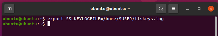
This command, will instruct the OS to store all sessions keys in a file named tlskeys.log in the home folder of your user. there are a few things to note here;
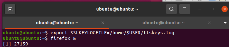
This commands will work for this terminal session only. Once the terminal session windows is closed, the TLS keys will not be stored in the log file anymore. The storage of these keys applies to TLS keys of this process and all processes spawned from it only. this means that after running the command, if you start your browser from the GUI, the keys will not be stored. You need to start the browser from within the commands line. Before you do that, start capturing the traffic in Wireshark.
Now start your browser (such as Firefox) from the command line:
firefox &
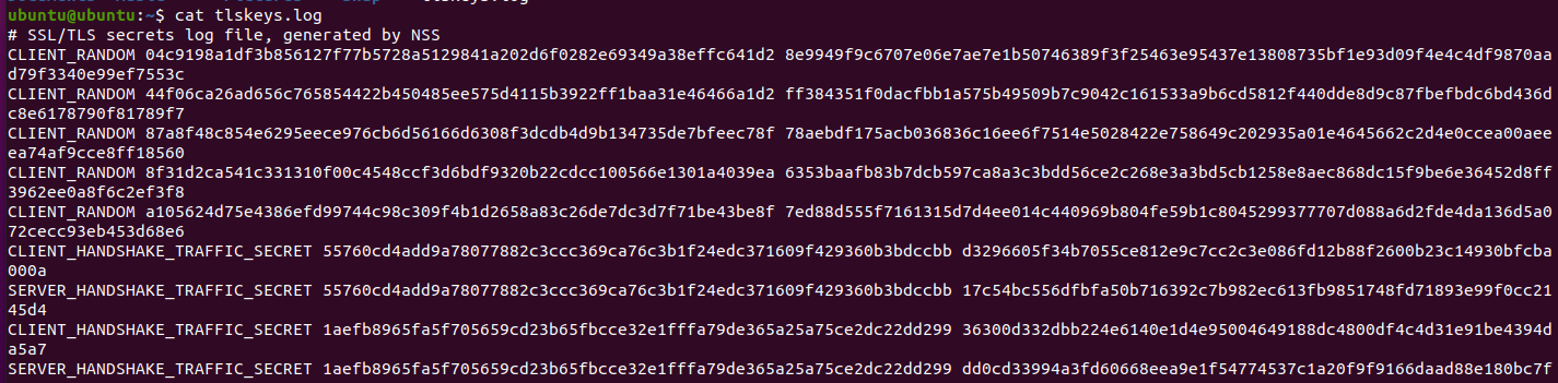
Visit an HTTPS based website like, google.com and go through searches or even try to sign in. Then, stop the packet capturing, and take a look at the tlskeys.log file.
cat tlskeys.log
You’ll see a few session keys for each session. It’d probably look something like this:
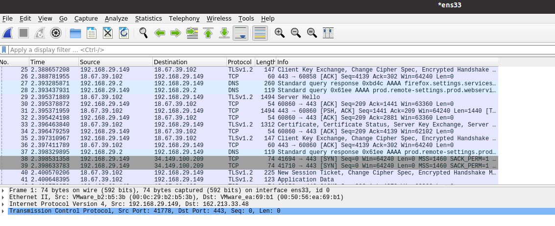
Now, if you look at the traffic captured by Wireshark, you’ll see that it is encrypted, like this:
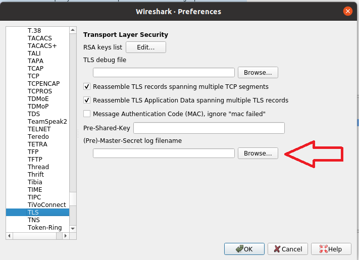
To use the TLS keys to decrpyt this traffic, go to Edit >> Preferences >> Protocols, and scroll down to get TLS. In the last field in the windows, you’l see “Pre-MasterSecret log filename”, click on “Browse…” next to it, and show Wireshark the location of the tlskeys.log file. Then, click “OK”.
Now, you’ll notice that the previously-encrypted TLS payload is now decrypted (mostly into HTTP2).
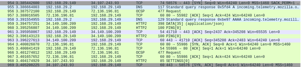
You’ll see that you’ll be able to extract a lot of HTTP objects that were not accessible before because of encryption.